Sunday 15 March 2015

Logistic Regression#Newton's_method#Derivation


Overview:

1. Introduction
2. Intuition for Sigmoid function (Hypothesis)
3. Cost function (Maximum Likelihood)
4. Optimization model: Newtons model
5. Derivation for Gradient and Hessian


Lets Begin:

This section is going to be a bit of mathematics. While the Logistic regression can be built just by using the formula, nevertheless it is worthwhile to look how the formula came into being. In this section "Logistic Regression Part-I" we will complete all the math required to understand the logistic regression and in the next we will learn few concepts and implement logistic regression to solve real world problems.


Introduction:

Logistic Regression as the name says "Regression" is not actually a regression technique but a classification technique. Classification is a technique in which you find the probability of an occurrence. For example, suppose you have a set of emails labeled as spam and not spam and you build a classifier using these emails as your training sample. With the influx of a new email your classifier will assign a probability value for the email being spam and not a spam.
Logistic regression is not confined to single class classification. It can be stretched to multi-class classification too. For the sake of simplicity lets just consider a single class classifier.

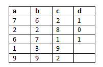
 The data-set to the right comprises of "m" training examples (each row) and "n" features (each column). All the rows are labeled as either 1 or 0. For the time being consider it a spam/not-spam training data-set with each example labeled as spam (1) and non-spam (0).


Intuition for Sigmoid function (Hypothesis):

If we recall the blog post on linear regression, for details look here. We know that our hypothesis (h) is defined as: 
                                hθ(x) = θ0 + θ1x1 + θ2x2 + .........θnxn

If you look at the hypothesis, you would see that for any random value θ or x the hypothesis may get any value ranging between -to +∞. But a probability model can only have values between 0 and 1. So what do we do? In-order to convert the hypothesis into a probabilistic model we use the sigmoid function

Sigmoid Function is a S-shaped curve which is also the special case of a logistic function and hence the name logistic regression is derived.


Sigmoid Function


The above graph is taken from Wikipedia, I would encourage you to go and read more on Sigmoid function on Wikipedia or elsewhere to have a more detailed understanding.

Applying sigmoid function to our hypothesis, we transform our hypothesis into the below form.
where   θT xθ0 + θ1x1 + θ2x2 + .........θnxn

"Voila, we have derived our hypothesis now. What we need now is the cost function and an optimization method to find our optimal parameters. We can always use gradient descent to converge the curve and find the parameters, but we have seen that already here. Going further we shall see a much better approach known as the newton's method to find the optimal parameters"

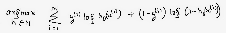
Cost function (Maximum Likelihood):

Before going into the derivation let us have a quick look on how the cost function of the Logistic Regression model looks.
Now, this is a heck of an equation, by just looking at it one would be confused. The whole formula is nothing but a representation of "Maximum likelihood" for logistic regression.


What is a maximum likelihood estimation?
"The notion on maximum likelihood is that the hypothesis you derive is likely if it makes what you see likely. It is the one that maximizes the probability of the data given the hypothesis."


hML: stands for the maximum likelihood. The above equation says to select a h (hypothesis) among all the H (hypothesis) that maximizes the probability of the actual data or (y).

Since all the data point (y) are independent of each other, the total probability would just be the product of all the independent probabilities given as below. 


We know that our hypothesis in discreet, which is, either 1 or 0, we model our yi as Bernoulli's random variable. Therefore using Beroulli's principle on the probabilistic model we get the following equation.


 Now we substitute the probability model in our maximum likelihood equation.


Probability of products is computationally difficult, therefore we perform the logarithmic of the whole equation . The advantage of using the logarithm is that the product converts into summation which is easier to deal with and also, log in an increasing function. For example, if you plot a log function of x, increasing x would also increase log(x). Though the values may change as a larger increase in x would result in small increase in log(x) but the maximum doesn't change or the sequence doesn't change. In probabilistic model we are not interested in the values but the candidate that generates highest probability. This candidate would be same for x and log(x).

We use the log properties of multiplication and exponent and compute the above equation. 


The above equation shows the formula that maximizes the likelihood (going up hill all the way to the top in the curve). However, finding the local minima is easy in our case cause we have seen optimization techniques like gradient descent that converges to the minimum point. Therefore we convert the whole equation into local minima by prefixing the equation with a -ve sign.

The equation we obtain above is our cost function for Logistic regression. We now just average the whole to get to the minimum value and get out final cost function as:


"Now that we have derived out cost function, let us go ahead and derive the gradient. Surprisingly, you will find that the gradient for both linear regression and logistic regression are the same."


Optimization model- Newtons model:

The Newton method is an advanced optimization method. If you recall the Gradient Descent approach, you will find that the parabolic curve converges or (the minimum cost function) is found after performing the algorithm for many iteration. The iteration can, in some case, be 1000's or even cross 10000's which is time consuming and costly. Reason for such delay is because in Gradient Descent approach the slope of convergence in too small. However, in Newton's method the minimum f(θ) (cost function for logistic regression) can be reached in few iteration. 

 Intuition:  

The Newton's method takes the tangent from any point in the curve and set the value for the new  theta when the tangent meets the x axis (theta axis). This process continues until the minimum f(θ) is reached  

From the Graph at the right we see that at θ3 the f(θ) is minimum. Looking at the plot it can also be understood that the curve converged in just three iteration (θ1,θ2,θ3,) which is very less.

Now lets go ahead and write the complete formula of convergence for using Newton's method.
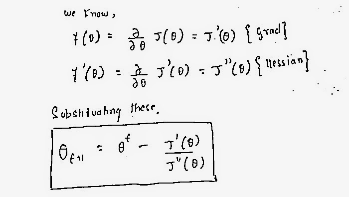


 Note:
J'(θ) is the Cost function for Logistic Regression
J''(θ)  is the Hessian.


Derivation of Gradient and Hessian:

Taking the derivative of the cost function in terms of theta would give us our Gradient. 

Gradient:


So now that we have derived the formula for gradient, let's use it and derive the Hessian for Newton's method. 

Hessian:

"For the time being, let's only know that Hessian is the double derivative of the cost function."


Thursday 19 February 2015

Introduction to Machine Learning


 I guess, most of us have watched the movie "I-robot", if not please do watch, it is indeed an awesome movie. Well what happens in that? Scientifically it shows artificial intelligence implanted into Robots that could perform tasks that are normally performed by human beings. Humans are often susceptible to errors, but robots or machines aren't they do what they are asked or what they are instructed. There may be a case in which by reiterating a process the machine may learn from its previous experiences and start performing or delivering with more accuracy.

Machine learning is a sub-field of Artificial Intelligence, probably the biggest field under it.


What is machine learning? 
 
Well, we can always refer the web to find the precise definition of machine learning. For me, machine learning is building algorithms that build a model (program) probably the best one by constantly learning from the data sets. The program or model generated is then used to make prediction. Machine learning is automating automation.


Normal programming: In normal programming systems we have inputs and we build a program using logic and then use the program for the inputs to get the desired results or output.
This is automating a process. You write a program once, send inputs to it and find the output.
What if the structure of the input data is varying constantly. We would have to write different programs for different structures of input data, which is tedious and time consuming. So what do we do, we call for help!


Machine Learning: Using machine learning techniques we build algorithms that takes the input and build the best program based on the input data. This program is then used on other input data to get the output. This is automating an automation.

The algorithm you write will automate the process of finding different programs or models for different input stream and then use the program that would find the output from the new input stream.


Components of Machine Learning:
Almost every machine learning problem has three components and we will discuss them now.

Representation: Representation is how do you represent the solution to your problem. For example suppose you were asked to find the Fibonacci series. You would either use c or c++ or Java or other languages to build a program that would do your task. Similarly in machine learning we have many different approaches (Decision Tree, Neural Networks, Naive Bayes, Support Vector Machines, Rules, Instances, Regression) o a problem. These approaches are the representation.


Evaluation: Evaluation can be told as the measurement of how better or accurate your approach is. You have written a program and now you evaluate how awesome it is. For example, out of 100 spam messages how many of the messages were declared as spam by your program or the prediction by your program is how close to the actual output. Different evaluating models are Accuracy, Precision and Recall, Squared error, Likelihood, Entropy, Posterior probability and others.
   

Optimization: We have different representations, different Evaluation strategy for a problem and each different combination could result in n numbers of outcomes. Optimization helps us to search the best outcome or best fit to the problem. Optimization is the strategy that picks the best program. Different optimizing approaches are Greedy search, Gradient descent and etc.


When combining these three components a whole system of machine learning is developed.

A simple combination can be:
Regression (Representation)-> Squared error (Evaluation)-> Gradient descent (Optimization).


Types of Learning:

There are different types of datasets, for example, some datasets have labels, some don't and some have partial labels. There is a heavy dependency of employing an algorithm based on the type of the data-set. 

Some different types of learning are:

Supervised Learning:  Supervised Learning is a type of learning in which you have supervision. For example, you know if the message is spam or not. In technical terms all the instances (rows) of the dataset are labeled or they have a class (output). 

Unsupervised Learning: Unsupervised Learning is a type of learning where you don't have supervision. For example, you do not know if the message is spam or not. All you have is a set of attributes and their values. Based on the attribute value you have to segregate the spam and non-spam messages. A good example for Unsupervised learning is server clustering. In server clustering, for each server you may have different attributes like the RAM, CPU space, CPU load and others. There is no specific class (output) for the input data-set. In such a case one has to group different servers based on their similarity in space, performance, speed and other attributes.

Semi-Supervised Learning: Semi supervised is a combination of Supervised and Unsupervised learning. Here we have supervision on partial data-set i.e, some are labeled and some are not. In practical applications there are many cases where 80% of the messages are not labeled as spam or not-spam. Such a scenario spawns the importance of Semi supervised learning where the messages are segregated as spam or non-spam based on the labeled data (20%) using supervised learning technique and then unsupervised learning is applied on the other data (80%). Based on their similarity with spam or non-spam messages- computed using the labeled data, the data-sets are classified into spam or not-spam.

Now let us understand each of them with  layman's examples:

Lets suppose we have a data-set as given in the RHS. What do you think of the data set. 
The data set can have different view.

1. One can say that column a,b,c are different attributes and d is the outcome of each instance (row).
2. One can also say that a,b,c and d are all attributes.


Intuition 1: If you see conscientiously you will see a pattern in the above data-set, which is, if you multiply 3 to each a, b and c and add them you will get d.
2*3 + 2*3 +2*3=18 
3*3 + 3*3 + 3*3=27
Therefore, we can build a model and use the model on our future data set to predict the outcome.Now, if you get a new row with columns a,b and c. 
We can easily predict d.

If the new instance is a=5, v=1 and c=3 one can perform the logic and find the outcome. i.e d= 5*3 + 1*3 +3*3= 27. Here 27 is the predicted call for the new instance.

This kind of learning is generally called Supervised learning. 


Intuition 2: The above data-set also exhibits a different pattern. If you observe closely you might argue  that the instances in the above data-set can be divided into even and odd rows. Where rows 1 and 4 are even and rows 2 and 3 are odd. So instead of building a pattern to calculate the d's output, we build two cluster and say if all the attributes a, b, c and d are even then they fall into the even cluster, else they fall into the odd cluster.
For example : suppose we get a new instance as shown in the RHS.  

Which cluster would the instance fall? Odd because all the attributes value are odd.

This kind of learning technique is called as Unsupervised Learning.


Intuition 3: Data-set can also be partial, for instance some of the data set is labeled and some aren't labeled. In such a case neither supervised or unsupervised learning would be handy. 

Let say we have a data-set similar to the data-set plotted in the RHS. The column d is absent for the 4th and 5th row. So how do we learn the data-set. In this case we use partially supervised and partially unsupervised learning. Looking at the data-set what pattern do you see? Can we say, If a>5, b>5 and c<5 then d=1. Similarly, If a<5, b<5 and c>5 then d=0, which is  but supervised learning. 


Similarly, we can group the whole data set into 2 groups. 
Group 1: a<5, b<5 and c>5
Group 2: a>5, b>5 and c<5

Based on our grouping, now we can apply unsupervised learning on the 4th and 5th row and classify (label) them as 1 and 0.


After we are done with the labeling we get the complete data set. Now we can apply whatever algorithm or learning we want to the new incoming data-set or new instances.


Thought for the Blog:

"Labeled data is scarce and expensive to obtain, whereas unlabeled data is abundant and cheap. With the shortage of labeled data enterprises are employing and building systems upon the unlabeled data to gain intelligence out of their data-set. However, it is assumed that a labeled data can give more insights than a unlabelled data.
Therefore many real world application today are heavily engaged with semi-supervised learning  techniques."

In many cases the learning from both unlabelled and labelled data can result in better result in the development of better models than learning each of them separately would.